
Introduction to DSP
Digital Signal Processing (DSP) is a technique used by engineers to analyse and process digital signals. Signals in this case are streams of analogue or digital data. The main applications of DSP are audio signal processing, data compression, digital image processing, video compression, speech processing, speech recognition, digital communications, RADAR, SONAR, seismology, biomedicine and many others. DSP is used in everyday technology without you even realising it. For example, when you make a long-distance call the fact that there is no noise and no echo on the call is because DSP technology is being used to remove them. Data correction and compression in data communications are in fact the cornerstone of the internet speeds we are used to today. MP3 is a term that most people are familiar with today. What most people are unaware of is that MP3 is a collection of DSP technologies standardised for the compression of music. The technology is pervasive yet still not widely understood and applied to disciplines outside of engineering.
The technology has various tools for separating the parts that make up a signal. Signals are themselves made up of multiple signals. Fourier theory shows that signals like those for sounds, however complex, can be represented as the sum of an (infinite) number of sine waves.
In the example below a slow-moving wave is added to a faster-moving wave and creates a new wave which is a combination of both. In DSP terminology, each wave has a different frequency and amplitude, the frequency being the timings of each wave hump and the amplitude being the height of each hump.

The graphic on the front page depicts how waves of different frequencies and amplitudes can be successively added to create a new wave which starts to look increasingly like a price series.
One of the main uses of DSP technology is to take waveforms and extract their component waves. In the case above, the C wave would be decomposed into separate the A and B waves. The way waves can be added together is called superposition and has application in many other fields. So in the example of noise removal on a telephone call; noise is normally high-frequency waves which can be separated from the original signal by decomposing the signal into its constituent waves, removing the high-frequency wave and then adding the waves back together to recreate the sound without noise.
DSP Techniques
In DSP, engineers usually study digital signals in one of the following domains: time-domain (one-dimensional signals), spatial domain (multidimensional signals), frequency domain and wavelet domains. Engineers choose the domain in which to process a signal by making an informed guess (or by trying different possibilities) as to which domain best represents the essential characteristics of the signal.
The field developed from Analogue Signal processing which has been around for some time and mainly implemented in hardware. An example of hardware-based signal processing is the use of graphical equalisers to change the treble and bass of audio. With the increasing use of computers, the number of applications for digital signal processing has increased as does the complexity and sophistication of the DSP algorithms.
Sampling
Many signals are continuous i.e. analogue. A sound for example is an analogue signal. So that an analogue signal can be processed by a computer it must first be converted into digital signals.
To convert an analogue signal to a digital signal the signal has to be sampled. Sampling involves taking discrete values from the continuous-time signal at equidistant time intervals. The sampling should be at a level such that the original signal can be reconstructed from the digital signal. Signals need to be sampled at the Nyquist frequency which is defined as twice the bandwidth of the original signal i.e. it has to be sampled often enough to be able to recreate the frequency but no more than that.
For example in the diagram below the lines represent sampling points.

A digital value of the amplitude (or the height) is sampled at each point and stored as a sequence of numbers. Sampling is used to convert analogue sound into digital sound for compact disks for example. The sampling rate for a digital sound recording is the number of times the amplitude is measured each second. For CD audio, this value is 44,100, which means that 44,100 data values are encoded each second, which can be written as 44.1kHz. (Hz is an abbreviation of Hertz — which means the number of times, or cycles, per second.) 44.1kHz recording enables good sound reproduction — the human ear is capable of discerning frequencies between around 20Hz and 20kHz so sampling outside of this range is not required. (The sampling rate for telephones is 8kHz.).
Time Domain
Most people are used to seeing signals in the time domain, i.e. events are ordered by time. For signals in the time domain, the most common DSP technique employed is called Filtering. With filtering, the signal is passed into a function which transforms the data into a new signal.
In the example below, an analogue signal is first sampled, then filtered, and then converted back into analogue.
Typically filtering is used to filter out or remove unwanted components in a signal. It could be noise or outliers. A filter can also be used to transform a signal into a different form. Digital music effects such as phasors and delays are examples of transformations. Filters are also used to attenuate (or amplify) certain parts of the signal.
Much of the DSP literature is dedicated to the design of filters and the engineer is often faced with requirements that are contradictory. For example, removing noise in audio which is high frequency might also remove other high-frequency components which are not noise as clicks and high pitched noises. All filter design is about finding an acceptable compromise to these conflicting requirements.
Frequency Domain
As well as viewing signals in the time domain, it is possible to also view them in the frequency domain. Time-based signals can be transformed into a set of frequencies and their phases.
This can be seen in the graph below. Note that the waves are shown as points because we are dealing with discrete digital samples of a wave.

The top left is a single sine wave. This corresponds to a single frequency which is shown as a point on the graph to its right. So one wave corresponds to one point in the frequency domain. The next graph down is a second wave with a different amplitude and frequency. This corresponds to a different point in the frequency domain. Recall from earlier that waves can be added together to create new waves, so adding the top two waves produces the bottom wave. When this wave is transformed into the frequency domain, this now corresponds to two points.
Signals are converted from time or space domain to the frequency domain usually through the Fourier transform (although there are other types of transforms). The Fourier transform converts the signal information to a magnitude and phase component of each frequency. It decomposes a function of time into the frequencies that make it up. This is similar to representing the sound of a musical chord by the loudness of each note played in it.
The frequency domain holds the same information as the time domain so it is possible to go from the frequency domain back into the time domain. This is called the Inverse Fourier Transform.
In the diagram below, a simple sine wave shown by the green curve has random noise added. Random noise is composed of many different high-frequency waves. This is shown by the blue curve. When a Fourier Transform is applied, the result is the red curve.
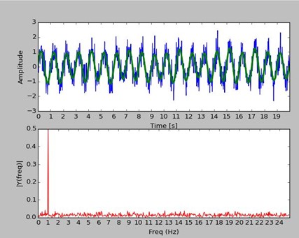
The frequency of the original green curve is easy to spot in the red plot because it has the highest amplitude. The green curve can be recreated by removing all other frequencies which have an amplitude lower than a threshold, say 0.1, and then doing an Inverse Fourier Transform. The result is the green curve.
Summary
The field of DSP is vast and in constant development. The ideas presented above barely scratch the surface of the field. However, enough has been described to give the reader enough understanding for the next section.
The main concept to take away is that DSP has many tools and techniques for the analysis and transformation of signals. Filtering and the use of frequency domains presented here are two techniques which are widely applicable to many DSP problems.
Application of DSP to Price Analysis and Trading Systems
DSP is a natural choice of toolset to the analysis of prices because prices are already in the form of a time-domain signal sampled at a specified time interval. Daily prices for example are discrete-time samples of a more continuous time series. Observation of market behaviour shows cycles with rising and falling prices. Sometimes price changes are slow equating to low frequencies or fast equating to high frequencies. Using various DSP concepts, interesting discoveries can be made about the data. Consider the following example:
This graph shows the returns for corn over the last 20 years. It doesn’t look like a price series because the returns are not accumulated. The reason for this is that in order to analyse market data using DSP tools we want to treat each price as a discrete-time sample rather than one sample referencing the previous samples.
What can we understand by looking at this data in the chart? Initially, not very much. We can see that the range of returns is greater in recent times but that’s about it.
Transforming the data using the Fourier Transform converts it to the frequency domain:
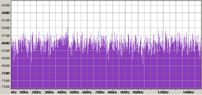
Recall from earlier examples that repeating signals which are like sine waves would produce peaks in the frequency domain. In this example, we are seeing no individual peaks. Instead, there is a wide range of frequencies with no concentration or groupings. This tells us some interesting facts that the time domain does not. With a market like Corn, it would be interesting to see if there was a dominant cycle from effects such as weather. Clearly, from this example, the number of frequencies is spread quite widely and there is no obvious dominant frequency. This tells us that repeating consistent frequencies in market data are not common and this result is the same for many other markets.
As fund managers, we are interested in frequencies that correspond to trends. We have developed proprietary signal filters to extract trend strengths at multiple frequencies.
When we run one of the filters on the Corn data the result is shown below. Trend strengths are shown in the vertical axis.

When you look closely at the price data and compare it to the trend strength captured we see that the higher strength corresponds to directional moves. But how can we evaluate how effective this filter is? Has it extracted the correct frequency? Are the start and ends of the trend have close proximity to the start and end of changing trends’ strengths from the filter? Is there any way we can improve on it?
DSP technology has a range of techniques used to design and refine filters. One of the most useful techniques is to look at the results of a filter in the frequency domain.
Recall from earlier discussions that theoretically a single wave would result in a single point in the frequency domain. So by viewing the result in the frequency domain we can see how many frequencies are now present after the filter operation and, most importantly, what their magnitude is.
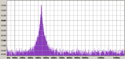
The result above shows the frequency domain plot on the Corn data after the filter has been applied. What this immediately shows is that one frequency has been amplified and the others reduced. This is the trend frequency we are interested in. It can also be seen that frequencies that are adjacent to the target frequency have been amplified but to a lesser extent. What this shows is that the filter is not perfectly isolating one frequency. If it had done a perfect job it would be a vertical line with no adjacent frequencies. So why is this? Despite the sophistication of filter design techniques, no filter is perfect and certain compromises must be made in the design.
Filter design suffers from the Uncertainty Principle. This principle states that it is impossible to accurately identify the location AND the frequency with equal precision. It has parallels with the Uncertainty Principle in Quantum Mechanics[1]. In other words, the more accurately you know the frequency the less accurate your location measurements are and vice versa. This is a physical and theoretical limit that cannot be solved. This creates a significant problem for the filter designer which can only be overcome by compromising certain filter design objectives.
We have been working on the design of our filters for some time using DSP tools to optimise the design to deal with these compromises. The frequency plot above shows what the filter looks like following good design principles. So, what does a bad filter look like?
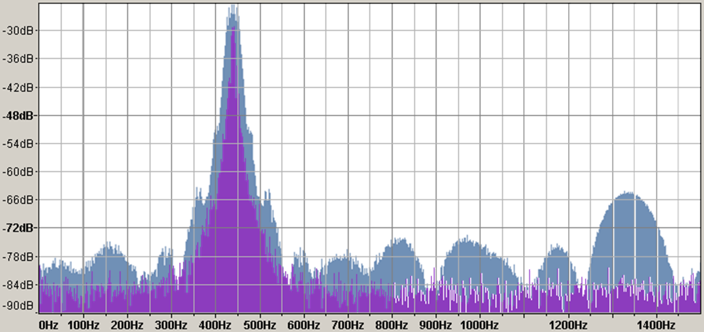
A bad filter is shown by the blue plot above. This is the frequency domain plot for a simple moving average. Simple moving averages are a primitive type of filter and are commonly used for systematic trend following systems.
What are the features on the blue plot which tell the filter designer that it is a worse filter than the purple plot? The first thing you notice is that although the frequency identified is the same, the breadth of adjacent frequencies is wider meaning that it is including more frequencies in the result. The effect of this in an actual trading system is that the trend strength will be higher for longer causing the filter to have more lag. The other key feature that you notice is the prominent humps on either side of the target frequency. These are known as “side lobes” in the literature. These show amplification of frequencies that are nowhere near the target frequency. These frequencies arise as an unwanted feature of the implementation of moving averages. These are essentially fake responses to a frequency which are not present in the data that are caused as a side effect of the implementation. In trading systems, these manifest as false signals and whipsawing.
From this example, we can see that our filter is an improvement on a simple moving average. The improvements in the design are matched by improvements in the strategy performance in research results.
The poor performance as a filter of moving averages is further exacerbated when more than one filter is used. Many trend-following systems use multiple moving averages with different periodicity and then sum the results to get a combined signal strength. This has the effect of summing the errors as well as the frequencies which magnifies the errors in the filter.
Without an understanding of filter design, the uninitiated can make incorrect assumptions. For example, one assumption could be that more filters are better. Would 2 filters be better than one? Would 10 filters be better? Without DSP technology there is no framework for intelligently making this decision. Because of the compromises made in filter design, adding more filters can increase the overlap of the frequency response. When building trading systems that have many moving averages, it is possible to unwittingly increase the response to a single frequency rather than increasing the breadth which was likely the original goal.
Conclusion
DSP technology gives us a framework for building better systems. The approach has enabled us to develop systems that have improved lag and better frequency isolation. It has also enabled us to build systems that are free of undesirable artefacts in the implementation which may cause invalid trading signals. Without a design framework, there is a tendency for the uninitiated to resort to curve fitting. Using a framework such as this, we have been able to evaluate and improve our models using tools that are independent of strategy returns. This is approach is more likely to result in robust systems that are not curve fitted to transient market behaviour.
This has served to be a guide on some of the concepts of DSP and how they are applied. However, the field of DSP is vast and with a steep learning curve for people outside the field. This guide is merely an introduction to a few simple concepts in DSP to give the reader some insight into our methodologies. The exact nature of the use of DSP in our systems is not disclosed and additional techniques and methodologies have been developed based on DSP in the development of our signalling methodology.
[1] When applied to measuring an electron for example the speed and the location cannot be identified with equal precision.